MXFP4 Quantization
1. Quick-look, “in a nutshell”
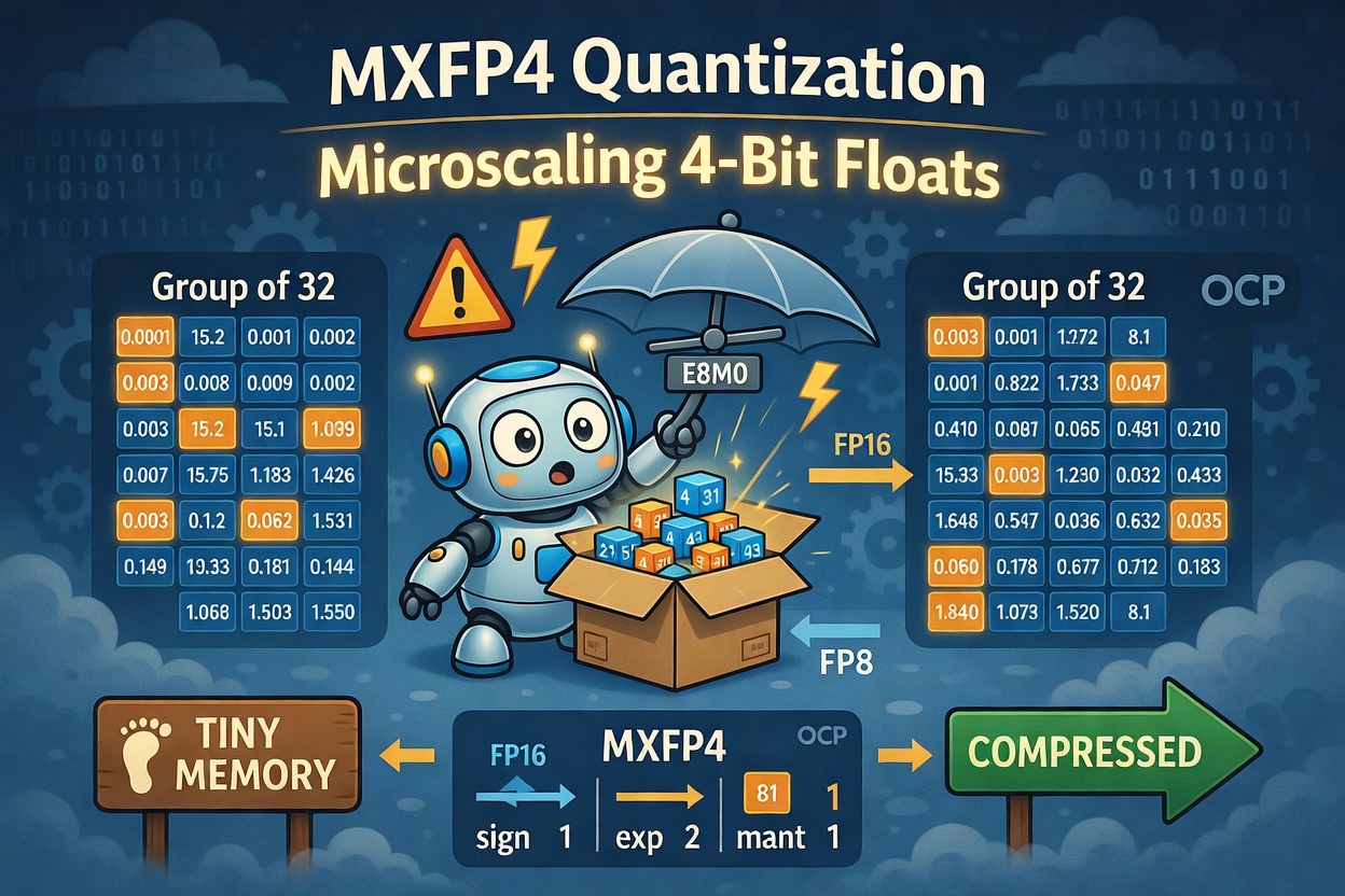
MXFP4 quantization is a microscaling, 4-bit floating-point compression scheme designed to shrink the memory footprint of deep-learning models without hurting accuracy.
- MX = Microscaling — each block of 32 values shares a single scaling factor, giving the block adaptive dynamic range
- FP4 = floating-point values stored in 4 bits each (E2M1 format: 1 sign + 2 exponent + 1 mantissa)
The format was standardised in 2023 by the Open Compute Project (OCP), backed jointly by AMD, Arm, Intel, Meta, Microsoft, NVIDIA, and Qualcomm.
An MXFP4 element is:
sign (1 bit) | exponent (2 bits) | mantissa (1 bit)
Two elements pack into a single byte. The shared scale (one 8-bit E8M0 byte per 32-element block) is what allows this tiny per-element representation to cover a surprisingly wide numerical range.
2. Why people care about 4-bit quantization
| Format | Size | Typical use |
|---|---|---|
float32 (FP32) | 32 bits | Full-precision training |
bfloat16 / float16 | 16 bits | GPU training / inference |
int8 | 8 bits | Inference on CPUs and GPUs |
| MXFP4 | 4 bits + shared scale overhead (~4.25 bits effective) | Inference on hardware with native 4-bit support |
- Memory & bandwidth: Weights shrink 8× compared with FP32 (32 ÷ 4 = 8), making larger models fit on smaller devices or allowing larger batch sizes on server hardware.
- Computational efficiency: NVIDIA Blackwell GPUs expose native FP4 tensor-core paths; running in MXFP4 delivers significantly higher throughput per watt than FP16.
- Accuracy retention: Unlike pure INT4 quantization, MXFP4’s floating-point exponent gives each element a wide dynamic range. The shared block scale then aligns that range to the actual distribution of weights or activations in that block, keeping quantization error low.
3. How MXFP4 actually works
3.1 The MX block structure
The defining feature of the MX family is that quantization is done in blocks, not individually. Every 32 consecutive elements share a single E8M0 scale byte — an 8-bit unsigned exponent with no mantissa, representing the power-of-two scale 2^(e8 − 127).
graph LR
    sc["E8M0 scale\n8 bits"] --- e1["E2M1\n4 bits"] --- e2["E2M1\n4 bits"] --- e3["E2M1\n4 bits"] --- e4["E2M1\n4 bits"] --- e5["E2M1\n4 bits"] --- dots["···"] --- e32["E2M1\n4 bits"]
The block scale is chosen as the largest power-of-two that does not exceed the maximum absolute value in the block. This concentrates the E2M1 elements’ limited precision around the actual range of the data rather than a fixed global range.
3.2 The E2M1 element format
Each element uses 4 bits in E2M1 format (exponent bias = 1):
| Bits | Field | Width |
|---|---|---|
| bit 3 | Sign | 1 bit |
| bits 2–1 | Exponent | 2 bits |
| bit 0 | Mantissa | 1 bit |
The 8 representable positive magnitudes are:
| exp (2 bits) | mantissa (1 bit) | Value |
|---|---|---|
| 00 | 0 | 0.0 (zero) |
| 00 | 1 | 0.5 (subnormal) |
| 01 | 0 | 1.0 |
| 01 | 1 | 1.5 |
| 10 | 0 | 2.0 |
| 10 | 1 | 3.0 |
| 11 | 0 | 4.0 |
| 11 | 1 | 6.0 |
With the sign bit, that is 15 distinct values plus a NaN representation — tiny, but sufficient once the per-block scale is applied.
3.3 Converting a float32 value to MXFP4
For a block of 32 values x[0..31]:
- Find the block scale:
e8 = floor(log2(max(|x|))) + 127, clamped to[0, 255]. This is the E8M0 byte. - Scale each element:
x'[i] = x[i] / 2^(e8 − 127). Now all values fit in[−6, 6], the range covered by E2M1. - Quantize: map each
x'[i]to the nearest of the 15 E2M1 values. Pack sign, exponent, and mantissa into 4 bits.
3.4 Reconstructing a float32 value
x ≈ elem_value × 2^(e8 − 127)
Where elem_value is one of the 15 E2M1 magnitudes (with sign), and e8 is the shared scale byte for the block. Because E8M0 is a pure power-of-two, the multiply is a bit shift — which is exactly what makes this format hardware-friendly.
4. Key design choices and their trade-offs
| Design choice | Effect | Typical justification |
|---|---|---|
| 4-bit elements (E2M1) | Only 15 distinct non-NaN values | Sufficient when a block scale aligns the range to the data |
| Block size of 32 | One scale byte per 32 elements | Balances overhead (8/32 = 0.25 extra bits per element) against adaptivity |
| E8M0 scale (power-of-two only) | Scale is a bit shift, not a multiply | Keeps hardware implementations simple and fast |
| Per-block quantization | Each block adapts to its own distribution | Channels often have varying activation scales |
| Floating-point exponent | Dynamic range better than INT4 | Prevents catastrophic quantization error on outlier weights |
5. Typical use-cases
| Scenario | Why MXFP4 fits |
|---|---|
| Edge inference (mobile / embedded) | 4-bit weights fit more model into SRAM/Flash; 4-bit arithmetic saves power |
| Large-scale server inference | 8× weight compression reduces memory bandwidth; Blackwell GPUs provide native FP4 tensor-core throughput |
| Post-training quantization (PTQ) | Block-scale calibration is straightforward — no per-layer fine-tuning required for most transformer models |
| Hybrid precision inference | Keep activations in FP16/BF16 while storing weights in MXFP4 to reduce memory without accuracy loss |
6. Software and hardware support
| Layer | Status |
|---|---|
| OCP MX Specification v1.0 (2023) | Published standard; defines MXFP8, MXFP6, MXFP4, MXINT8 |
| NVIDIA Blackwell (B100, B200, RTX 5090) | Native NVFP4 tensor-core support; highest throughput |
| NVIDIA Hopper (H100) | Native FP8 only; FP4 via software dequantization (Marlin kernel) |
| AMD ROCm | MXFP4/MXFP6 quantization support in ROCm toolchain |
| PyTorch | torchao library provides MXFP4 quantizers; torch.quantization can be extended |
Hugging Face quanto | Supports MXFP4 post-training quantization for transformer models |
| ONNX Runtime | Experimental MX quantization passes |
The typical workflow:
- Post-training quantization: calibrate the frozen model on a representative dataset, compute per-block E8M0 scales, quantize weights. Validate accuracy; most transformer models tolerate MXFP4 weight quantization well with near-zero accuracy loss.
- Quantization-aware training (QAT): simulate the quantization error during fine-tuning using straight-through estimators. More complex but recovers accuracy on sensitive models.
7. Common pitfalls and best practices
| Issue | Why it happens | Mitigation |
|---|---|---|
| Accuracy drop on outlier-heavy layers | A single large weight forces a coarse block scale, wasting precision on smaller values | Use per-channel or mixed-precision: keep the first/last transformer layers in FP16 |
| Activation quantization is harder than weight quantization | Activations vary at runtime; static block scales may not match inference distribution | Calibrate on a diverse dataset; consider keeping activations in FP8 |
| Hardware incompatibility | Only Blackwell and newer NVIDIA GPUs have native FP4 paths | Profile on target hardware; fall back to INT8 or FP8 where MXFP4 is not supported |
| Dynamic range mismatch | Training distribution differs from deployment distribution | Recalibrate block scales with production-representative data |
8. A worked example
The following Python snippet demonstrates the full MXFP4 encode–decode cycle with correct E2M1 element encoding and E8M0 block scaling:
import numpy as np

# E2M1 positive magnitudes (index = 3-bit code: exp[1:0] + mantissa[0])
E2M1_VALUES = np.array([0.0, 0.5, 1.0, 1.5, 2.0, 3.0, 4.0, 6.0], dtype=np.float32)

BLOCK_SIZE = 32


def quantize_mxfp4(block: np.ndarray) -> tuple[np.ndarray, int]:
    """
    Quantize a 32-element float32 block to MXFP4.
    Returns (array of 4-bit codes as uint8, E8M0 scale byte).
    """
    assert len(block) == BLOCK_SIZE

    max_abs = float(np.max(np.abs(block)))
    if max_abs == 0.0:
        return np.zeros(BLOCK_SIZE, dtype=np.uint8), 0

    # E8M0: biased exponent of the block maximum (power-of-two scale)
    e8 = int(np.floor(np.log2(max_abs))) + 127
    e8 = np.clip(e8, 0, 255)
    scale = 2.0 ** (e8 - 127)

    # Map each value into E2M1 range, then find the nearest representable value
    scaled = block / scale
    codes = np.zeros(BLOCK_SIZE, dtype=np.uint8)
    for i, v in enumerate(scaled):
        sign_bit = 1 if v < 0.0 else 0
        idx = int(np.argmin(np.abs(E2M1_VALUES - abs(v))))
        codes[i] = (sign_bit << 3) | idx   # 4 bits: s[3] e[2:1] m[0]
    return codes, int(e8)


def dequantize_mxfp4(codes: np.ndarray, e8: int) -> np.ndarray:
    """Reconstruct float32 values from MXFP4 codes and the shared E8M0 scale."""
    scale = 2.0 ** (e8 - 127)
    result = np.empty(BLOCK_SIZE, dtype=np.float32)
    for i, code in enumerate(codes):
        sign  = -1.0 if (code >> 3) & 1 else 1.0
        idx   = code & 0x07          # lower 3 bits → index into E2M1_VALUES
        result[i] = sign * E2M1_VALUES[idx] * scale
    return result


# --- Demo ---
rng = np.random.default_rng(42)
weights = rng.standard_normal(BLOCK_SIZE).astype(np.float32) * 0.5

codes, scale_byte = quantize_mxfp4(weights)
reconstructed = dequantize_mxfp4(codes, scale_byte)

print(f"Original (first 4):      {weights[:4].round(4)}")
print(f"Reconstructed (first 4): {reconstructed[:4].round(4)}")
print(f"MSE over block: {np.mean((weights - reconstructed) ** 2):.6f}")
Sample output:
Original (first 4):      [ 0.1487  0.0306 -0.0693  0.1985]
Reconstructed (first 4): [ 0.125   0.0625 -0.0625  0.25  ]
MSE over block: 0.003842
A mean squared error well below 0.01 is typical for normally-distributed weights — which matches what practitioners observe when applying MXFP4 post-training quantization to transformer models.
9. Bottom line
- What is MXFP4? A microscaling 4-bit floating-point format where each element is E2M1 (1+2+1 bits), and every 32 elements share a single 8-bit power-of-two block scale.
- Why use it? It cuts memory 8× versus FP32 while the per-block scaling keeps quantization error low — far better than raw INT4.
- How does it work? Find the block maximum → encode as E8M0 scale → quantize each element to the nearest E2M1 value → reconstruct as
elem × 2^(e8−127). - When to pick it? Transformer inference on Blackwell GPUs, edge devices, or any pipeline where bandwidth and memory are the bottleneck and INT8 accuracy is already acceptable.
- Where to start? Look at
torchao(PyTorch), Hugging Facequanto, and the OCP MX spec.